Hyperbola
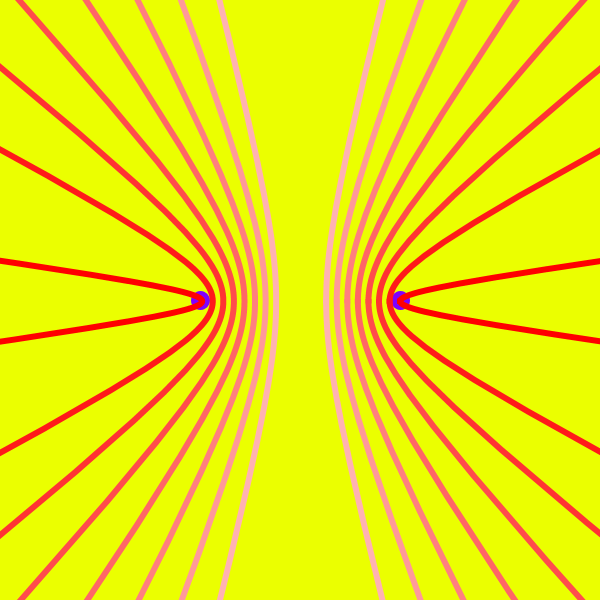
Clear[xc,xaalist,xcount]
xc = 1;
xcount = 7;
xaalist = Table[x, {x, .25, .99, (.99 - .25)/xcount}];
ParametricPlot[
 Evaluate@ Table[{a Sec[t], Sqrt[xc^2 - a^2] Tan[t]}, {a, xaalist}],
{t, 0.01, 2 Pi - 0.01},
 PlotStyle -> Map[Function[{Thickness[.01], #1}] , Table[Hue[0, i, 1], {i, .3, 1, (1 - .3)/xcount}]],
 PlotRange -> {{-1, 1}, {-1, 1}}  3  xc, Background -> Hue[0.18],
(* PlotLabels -> xaalist, *)
PlotLabels -> Placed[ xaalist, Left ],
 AspectRatio -> Automatic,
 Prolog -> {{Hue[.75], PointSize[.03], Point[{-1, 0}], Point[{1, 0}]}}]
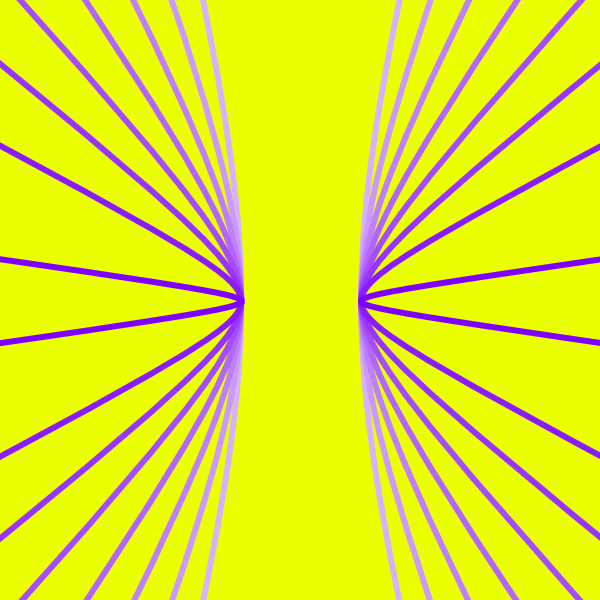
Clear[ xhformula, xelist, xhypers ]

xhformula[e_] := Function[{Sec[#], Sqrt[e^2-1] Tan[#]}] ;

(* a Sqrt[ e^2-1] == b *)
(* e = c/a for all conics *)

xelist = Table[ 1/x, {x,.25,.99, (.99-.25)/7}]

xhypers = Table[ xhformula[x][t], {x, xelist}]

ParametricPlot[
	Evaluate@ xhypers  ,
	{t, 0.01, 2 Pi -0.001 },
	AspectRatio->Automatic,
	PlotRange->{{-5,5},{-5,5}},
	PlotStyle-> Map[ Function[{Thickness[.01],#1}], Table[Hue[.75,i,1],{i,.3,1,(1-.3)/7}]],
	Background->Hue[.18],
	Axes->False
]
History
Description
Hyperbola describe a family of curves with single parameter. Together with ellipse and parabola, they make up the conic sections .
Hyperbola is commonly defined as the locus of points P such that the difference of the distances from P to two fixed points F1, F2 (called foci) are constant. That is, Abs[ distance[P,F1] - distance[P,F2] ] == 2 a, where a is a constant. GeoGebra: Two Ripples Traces Conics .
The eccentricity is a number that describe the “flatness” of the hyperbola. Let the distance between foci be 2 c, then eccentricity e is defined by e := c/a, and 1 < e. The larger the eccentricity, the more it resembles two parallel lines. As e approaches 1, the vertexes become more pointed.
The line passing through foci is the axis of the hyperbola. A line passing through center and perpendicular to the axis is the transverse axis. The vertexes are the intersections of the hyperbola and its axis.
Formula
- vertexes at {-1,0} and {1,0}
- eccentricity e
- (foci is {-e, 0} and {e, 0})
Parametric equation
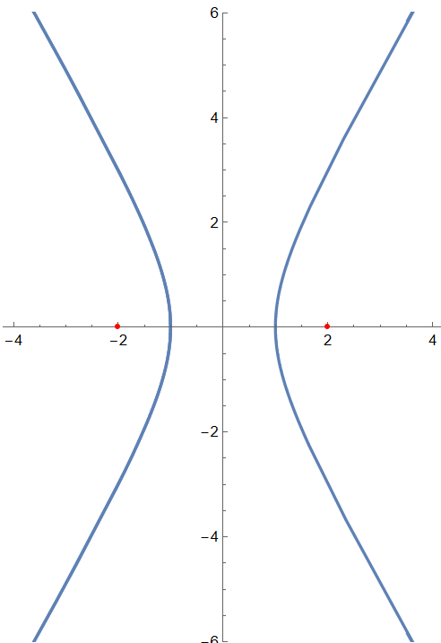
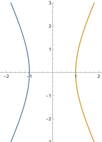
Clear[xecc]
xecc = 2;
ParametricPlot[{Sec[t], Sqrt[e^2 - 1]  Tan[t]}, {t, -5, 5},
PlotRange -> {{-1,1} 5, {-1,1} 6} ,
Epilog -> {Red, Point[ {-xecc,0} ], Point[ {xecc,0} ]}
]
Cartesian equation
Clear[ xecc ]
xecc = 2;
ContourPlot[ x^2 - y^2/(xecc^2-1) == 1 , {x, -5, 5}, {y, -6, 6},
PlotRange -> {{-1,1} 5, {-1,1} 6} ,
GridLines -> Automatic,
Epilog -> {Red, Point[ {-xecc,0} ], Point[ {xecc,0} ]}
]
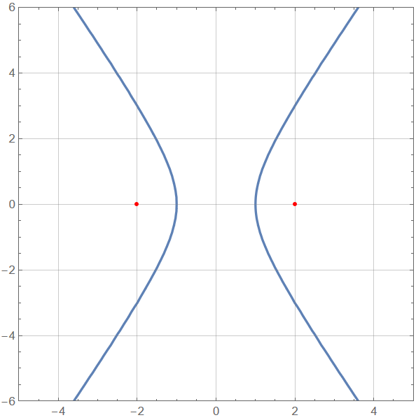
- vertex at {-a,0}, {a,0}
- directrix at
x == -a/e,x == a/e - asymptotes at
y== -b/a x,y== b/a x
Clear[ xa,xb ]
xa = 1;
xb = 2;
ParametricPlot[
Evaluate[ {{-xa Cosh[t], xb Sinh[t] }, {xa Cosh[t], xb Sinh[t] }} ] , { t, -2, 2},
 PlotRange -> {-3,3}
]
Cartesian equation
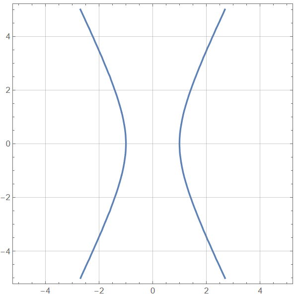
Clear[aa, bb]
aa = 1;
bb = 2;
ContourPlot[x^2/aa^2 - y^2/bb^2 == 1, {x, -5, 5}, {y, -5, 5},
 GridLines -> Automatic]
The parametric form with Sinh is derived by replacing y in x^2/a^2-y^2/b^2==1 with b*Sinh[t], then solve for x. This is analogous to the ellipse case where we replace a variable in x^2/a^2+y^2/b^2==1 by Cos[t] and solve the other to find {a*Cos[t],b*Sin[t]}.
Rectangular Hyperbola
- A rectangular hyperbola is a hyperbola with eccentricity Sqrt[2] ≈ 1.4142.
- Its asymptotes are mutually perpendicular.
- A simple Cartesian equation for rectangular hyperbola is
x y == 1
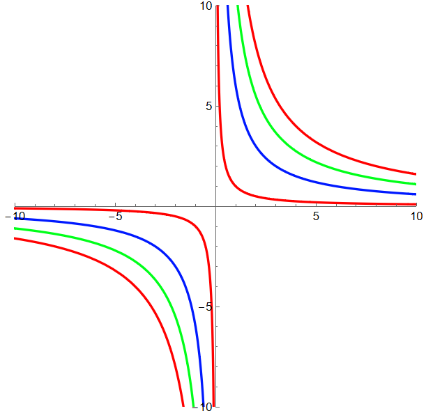
ParametricPlot[Evaluate@ Table[{t, i/t}, {i, 1, 20, 5}],
{t, -10, 10},
PlotStyle -> {Hue[0], Hue[.65], Hue[.35]},
 PlotRange -> {{-1, 1}, {-1, 1}} 10, AspectRatio -> Automatic]
- Rectangular hyperbola have the property that when streched along one or both of its asymptotes, the curve remains the same.
- That is, the curve {t, 1/t n}, {t n, 1/t}, and {t, 1/t} Sqrt[n] are the same curve with various degrees of magnification.
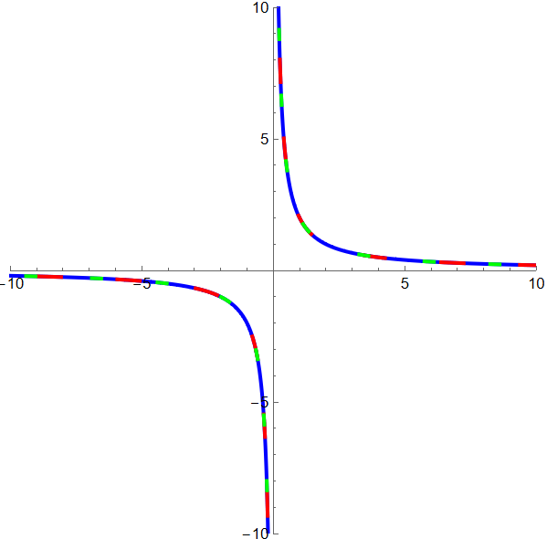
(* plotting 3 curves, with different colored dash lines, showing they overlap *)
Clear[n]; n = 2;
ParametricPlot[
{ {t, n 1/t}, {n t, 1/t}, {t, 1/t} Sqrt[n]},
{t,-12,12},
PlotStyle->{
{Blue, Thickness[.007]},
{Red, Thickness[.007], Dashing[{.05,.1}]},
{Green, Thickness[.007], Dashing[{.025,.1}]}
},
PlotRange->{{-1,1}, {-1,1}} 10,
AspectRatio->Automatic
]
Point-wise construction
This method is derived from the paramteric formula for hyperbola
{a Sec[t], b Tan[t]}
, where a and b are the radiuses of the concentric circles.
If a == b , then the curve traced is rectangular hyperbola.

- Let O be the origin. Let A and B be points on the positive x-axis.
- Let there be a circle centered on O and passing A.
- Let there be a circle centered on O and passing B.
- Let there be a line a1, that passes A and parallel to y-axis.
- Let there be a line b1, that passes B and parallel to y-axis.
- Let there be a point D on one of the circle.
- Let there be a line OD.
- Let A1 := Intersection[Line[O,D],a1]
- Let B1 := Intersection[Line[O,D],b1]
- Let there be a circle centered on O passing A1. Let the intersection of this circle and positive x-axis be E. Let there be a line g, passing E and parallel to y-axis.
- Let there be a line passing B1 and parallel to x-axis.
- The locus of intersection g and B1, as D moves on the circle, is a hyperbola.
Needs["PlaneCurveGenerator`"]

ListAnimate@ HyperbolaGenerator[{2, 1}, {0, 1.25}, PlotRange -> {{-2, 7}, {-2, 6}}, Ticks -> {Range[-10, 10, 2], Range[-10, 10, 2]}]
Optical Property
Light rays coming from one focus of a hyperbola refract to the other focus.
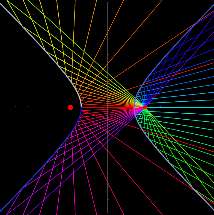
Needs["PlaneCurvePlot`"]

PlaneCurvePlot[{-Sec[t], Tan[t]}, {t, 0, 2 Pi, 2  Pi/50},
 CausticLineLength -> 30, CausticOrigin -> {Sqrt[2], 0},
 PlotDot -> False, PlotRange -> {{-4, 4}, {-4, 4}},
 CausticLineStyle -> Table[Hue[i], {i, 0, 1, 1/50}],
 Epilog -> {Red, Disk[{-Sqrt[2], 0}, 0.1]}, Background -> Black]
Pedal
The pedal of a hyperbola with respect to a focus is a circle.
Needs[ "PlaneCurvePlot`" ]

Clear[ecc, Hyperbola];
ecc = 1.8;

Hyperbola[ecc_] := Function[{-Sec[#], Sqrt[ecc^2-1] Tan[#]} ]

(* a Sqrt[ ecc^2-1] == b *)
(* ecc = c/a for all conics *)

PlaneCurvePlot[ Hyperbola[ecc][t],
{t, -Pi , Pi , (2 Pi )/50},
PedalPoint->{ecc,0}, PlotDot->False,
PlotCurve->False,
LineStyle->{RandomColor[ ]},
AspectRatio->Automatic,
Axes->False,
PlotRange->{{-1,1},{-1,1}} 2,
Epilog->{ {Hue[.7], PointSize[.02], Point[{-ecc,0}]} } ]
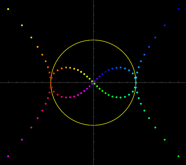
The pedal of a rectangular hyperbola with respect to its center is a lemniscate of Bernoulli
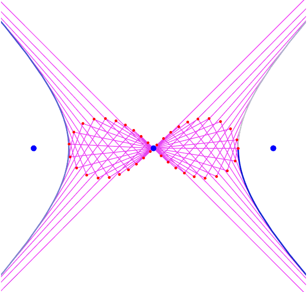
Needs[ "PlaneCurvePlot`" ]

Clear[e, Hyperbola];
e = Sqrt[2];

Hyperbola[ecc_] := Function[{-Sec[#], Sqrt[ecc^2-1] Tan[#]} ]

PlaneCurvePlot[ Hyperbola[e][t], {t, -3.14,3.14, 6.18/40},
PedalPoint->{0,0}, PlotDot->False,
LineStyle->RandomColor[],
AspectRatio->Automatic,
Axes->False,
PlotRange->{{-1,1},{-1,1}} 1.8,
Epilog->{ {Blue, PointSize[.02], Point[{-e,0}], Point[{e,0}]} }
]
Inversion
The inversion of a rectangular hyperbola with respect to its center is a lemniscate of Bernoulli.
Needs["PlaneCurvePlot`"]
Clear[ecc, Hyperbola];
ecc = Sqrt[2];
Hyperbola[ecc_] := Function[{-Sec[#], Sqrt[ecc^2 - 1]  Tan[#]}]
PlaneCurvePlot[Hyperbola[Sqrt[2]][t], {t, 0, 2  Pi, 2  Pi/54},
InversionCircle -> {{0, 0}, 1},
PlotCurve -> False,
DotStyle -> Table[Hue[tt], {tt, 0, 1, 1/54}],
PlotRange -> {{-1, 1}, {-1, 1}}  2.2,
AspectRatio -> Automatic,
Background -> Black
]
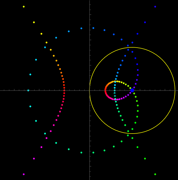
The inversion of a rectangular hyperbola with respect to a vertex is a right strophoid.
(*Inversion of rectangular hyperbola at the vertex*)
Needs["PlaneCurvePlot`"]
Clear[ecc, Hyperbola];
ecc = Sqrt[2];
Hyperbola[ecc_] := Function[{-Sec[#], Sqrt[ecc^2 - 1] Tan[#]}]
PlaneCurvePlot[Hyperbola[ecc][t], {t, -Pi, Pi, 2 Pi/(4 16)},
 InversionCircle -> {{1, 0}, 2}, PlotDot -> True, PlotCurve -> True,
 CurveColorFunction -> Hue, PlotRange -> {{-1, 1}, {-1, 1}} 3.2,
 DotStyle -> Table[{Hue[tt], PointSize[0.012]}, {tt, 0, 1, 1/(4 16)}],
 Background -> Black, AspectRatio -> Automatic]
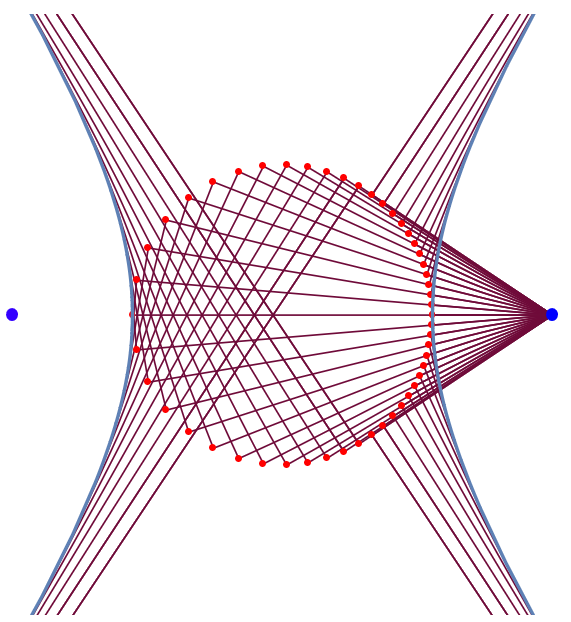
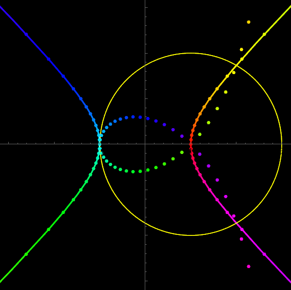
The inversion of any hyperbola with respect to a focus is a limacon of Pascal .
Needs["PlaneCurvePlot`"]
Clear[ecc, Hyperbola]
Hyperbola[ecc_] := Function[{-Sec[#], Sqrt[ecc^2 - 1]  Tan[#]}]
ecc = 1.7;
PlaneCurvePlot[Hyperbola[ecc][t], {t, 0, 2  Pi, 2  Pi/80},
 InversionCircle -> {{ecc, 0}, ecc}, PlotCurve -> False,
 DotStyle -> Table[Hue[tt], {tt, 0, 1, 1/80}],
 AspectRatio -> Automatic, PlotRange -> {{-1, 1}, {-1, 1}}  2.1  ecc,
 Epilog -> {Blue, PointSize[.02], Point[{ecc, 0}]} ,
 Background -> Black]
Quadric Surfaces
Equations of polynomials of degree 2 with 2 variables have cross sections that are hyperbola, ellipse, parabola in various ways.
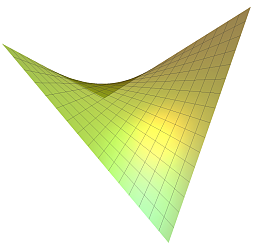 Hyperbolic Paraboloid
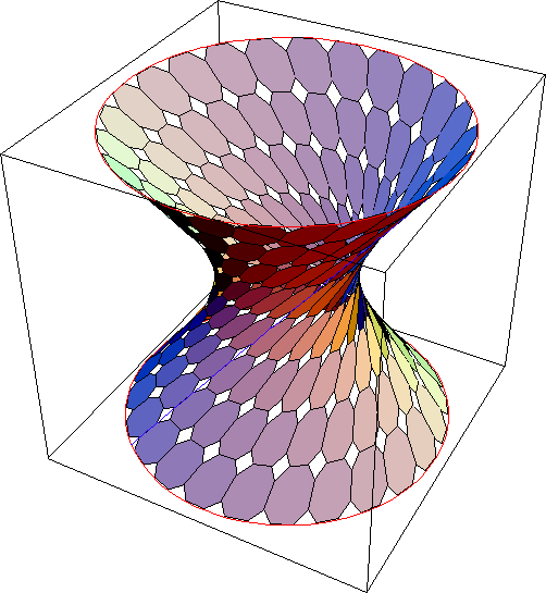 Hyperboloid of One Sheet
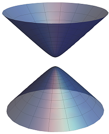 Hyperboloid of Two Sheet