Adaptive Sampling, Plotting Math Curve
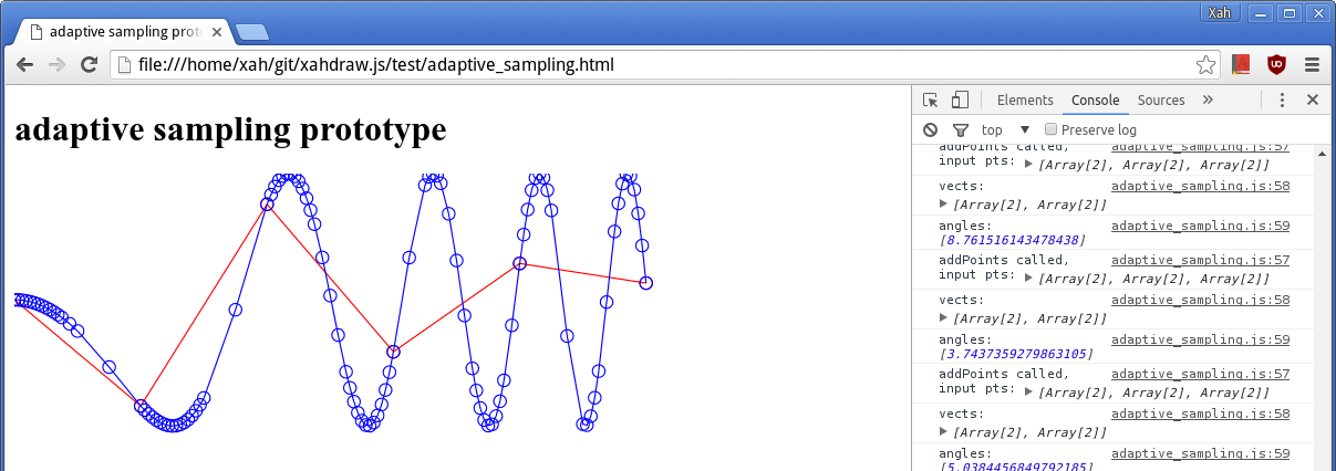
Sin[x^2]
from 0 to 5.
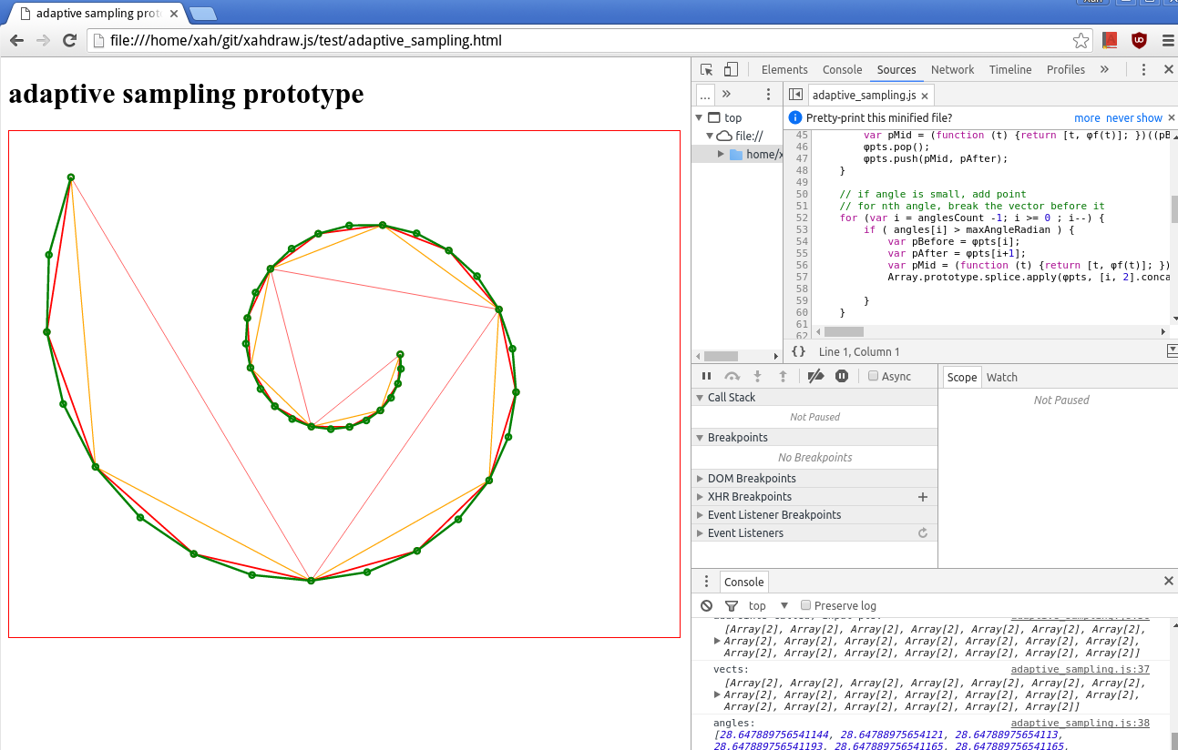
Red is initial plot of 6 points.
Blue is the final result.
Note that there are more points on the curve where the bend is sharp.
What is Adaptive Sampling?
Given a function, you want to plot it. The more points you use, the smoother the plot. But, points are wasted if the curve is fairly straight. So, you want adaptive sampling. You want to add points only when the bend is sharp.
If you use Mathematica, adaptive sampling is builtin in its Plot function. Likely, the algorithm is used in any quality 2D plot software.
But, for plotting complex plane, or 3D curves, a software may not have implemented adaptive sampling.
Why Do You Need Adaptive Sampling?
Adaptive Sampling is not just for saving storage/memory.
Adaptive Sampling is necessary because some curves will bend extremely sharply (small curvature) at some places, while fairly straight in other places. If you do equally distribute sampling, you'll miss out features of the curve at small regions where the curve jiggles and turn.
How to Implement Adaptive Sampling?
Start by plotting n equally spaced out input parameters. Let's say n = 5. For example, if x goes from 1 to 5, then you may start to plot at {1,2,3,4,5}.
Compute (x, f(x)) for each. To get a list of points (x, f(x)). Let's say your list is {P1,P2,P3,...}, where each is the coordinate pair {x,y}.
(note: each element actually should be {t,{fx[t],fy[t]}}), because it's more general and useful for parametric plot. But for simplicity of explanation, let's just say {x,f[x]}.
Each pair of neighboring points forms a vector. Compute the list of vectors. The first vector is P2-P1. The second is P3-P2, etc. Let's denote the list of vectors os {V1,V2,V3,...}.
Now, two neighboring vectors forms a angle. Compute all the angles. Let's denote the list of vectors os {A1,A2,A3,...}.
For thru the angles, if one of them is less than a predefined angle α such as 5 degrees, insert into the original points a midpoint on the vector (before) the angle point. (or the vector after the angle point) Make sure you do this for the last or first vector too, if it's neighboring point is greater than α.
Now, repeat the above
steps, until there are no angles larger than α, or, a recursion max count is reached.
. (we set a recursion max count, such as 5. Each time we go thru the step, we reduce it by 1. We need a recursion max count, because, for some curves such as Sin[x^2], the curve will have infinite number of sharper and sharper bends.)
Note: the above is easy to understand, but not an efficient implementation, because vectors and angles are computed redundantly for each recursion.
I had to implement it (in 2006) when doing a complex function plotter. see Stereographic Projection and Geometric Transformation on the Plane
note that, when you project a curve from a plane onto a sphere, if you don't have adaptive sampling, your sphere is going to look like a polygon ball, or not looking like a sphere at all. Because, on the plane, two neighboring points may be very close, but when mapped to the sphere, they may become wide apart. For example, you take a rope and wrap it on a big ball. The 2 endpoints doesn't show anything about the curve of the rope.